This page is outdated, please also see the man page.

How to run fdensity?

This mode allows measuring the density of functional annotations around the positions of a collection of QTLs. To illustrate how it works, first download the required example data:

The results from a full cis-analysis: TXT
The functional annotation for few Transcription Factor Binding sites: BED

Step1: Prepare the QTL data

First, you need to prepare a BED file containing the positions of the QTLs of interest. To do so, extract all significant hits at a given FDR threshold (e.g. 5%):


		Rscript ./script/runFDR_cis.R results.genes.full.txt.gz 0.05 results.genes

Then, transform the significant QTL list into a BED file using the following command:


		cat results.genes.significant.txt | awk '{ print $9, $10-1, $11, $8, $1, $5 }'  | tr " " "\t" | sort -k1,1 -k2,2n > results.genes.significant.bed

The resulting BED file looks like this:


		head results.genes.significant.bed

		1	15210	15211	1_15211	ENSG00000227232.4	-

		1	735984	735985	1_735985	ENSG00000177757.1	+

		1	735984	735985	1_735985	ENSG00000240453.1	-

		1	739527	739528	1_739528	ENSG00000237491.4	+

		1	754963	754964	1_754964	ENSG00000225880.4	-

		1	769222	769223	1_769223	ENSG00000228794.4	+

		1	832397	832398	1_832398	ENSG00000230699.2	+

		1	844342	844343	1_844343	ENSG00000223764.2	-

		1	879675	879676	1_879676	ENSG00000187634.6	+

		1	895705	895706	1_895706	ENSG00000187961.9	+

Note here that this file contains the follwing columns:

1. Chromosome ID
2. Start position of the QTL
3. End position of the QTL
4. QTL ID
5. Targeted phenotype ID (not used, can be whatever you want)
6. Strand orientation; this is important, you need to specify here on which strand the QTL has been mapped to

Step2: Run the density measurements

Now that you've got your QTLs ready to go, you can then measure the density using the following command:


		QTLtools fdensity --qtl results.genes.significant.bed --bed TFs.encode.bed.gz --out density.TF.around.QTL.txt

This generates a file density.TF.around.QTL.txt that contains the number of functional annotations per 1kb bins around QTLs.


		head density.TF.around.QTL.txt

		-1000000 -999001 1314

		-999000 -998001 1253

		-998000 -997001 1263

		-997000 -996001 1315

		-996000 -995001 1339

		-995000 -994001 1293

		-994000 -993001 1277

		-993000 -992001 1299

		-992000 -991001 1309

		-991000 -990001 1282

1. start position of the bin
2. end position of the bin
3. number of annotations in this bin

You can use the two following options to tune the calculations:

--bin [int]: size of the bin in bp (default is 1000bp)
--window [int]: size of the window around QTLs to be examined in bp (default is 1000000bp)

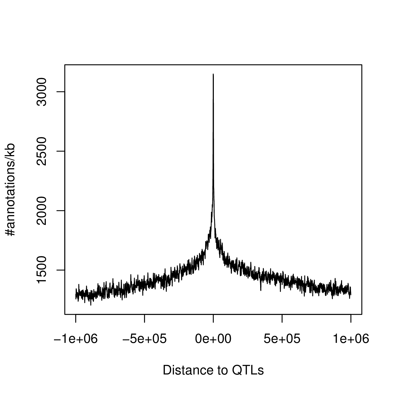
Once you've got your density measurements, you can plot them in R using:


		R> D=read.table("density.TF.around.QTL.txt", head=FALSE, stringsAsFactors=FALSE)

		R> plot((D$V1+D$V2)/2, D$V3, type="l", xlab="Distance to QTLs", ylab="#annotations/kb")

This is going to give you something like this:

Monday 11th July 2016